Update: The Baws Factor described in this post is now available in JASP >= 0.8.2.0 as "Inclusion Bayes Factor bases on matched models". So you don't have to calculate it by hand anymore!

JASP is a free statistics program developed by the group of Eric-Jan Wagenmakers at the University of Amsterdam. JASP is great for doing traditional null hypothesis testing: the kind of statistics that gives you p values.

But JASP is not a traditional program. It's a program with a mission. And its mission is to convince scientists to do Bayesian Statistics: the kind of statistics that gives you Bayes Factors.

A lot has been been written about Bayesian statistics, and much of that by people more knowledgeable than me. So I'll stick to a basic description of what a Bayes Factor is. And then I'll dive right into how you can apply this knowledge to a specific, but very common, kind of statistical test: a Repeated Measures Analysis of Variance, often simply called a Repeated Measures.

For this post, I'll assume that you know what a Repeated Measures is.

What's a Bayes Factor?

A Bayes Factor reflects how likely data is to arise from one model, compared to another model. Typically, one of the models is the null model (H0): a model that predicts that your data is purely random noise. The other model then typically has one or more effects in it, so it's (one of) the alternative hypotheses that you want to test (HA). If the data is much more likely to arise under HA than under H0, this means that there is strong evidence in the data for HA. This, in a nutshell, is the logic behind the Bayes Factor.

You can think of null hypothesis testing as one side of Bayesian statistics. A p value reflects the likelihood of the data (or data that is more extreme) given H0. But the likelihood of the data given HA is not factored into the p value, whereas it is factored into the Bayes Factor.

Now let's do a Repeated Measures with the bugs dataset that is included as an example datafile with JASP. Here, participants indicated how much they disliked bugs depending on how disgusting and frightening they are (the bugs, not the participants). It's set up as a 2 (disgusting: high v low) by 2 (frightening: high v low) within-subject design, so you can analyze it with a Repeated Measures.

Interpreting a traditional Repeated Measures

Let's first take a look at the traditional (null-hypothesis testing) Repeated Measures:

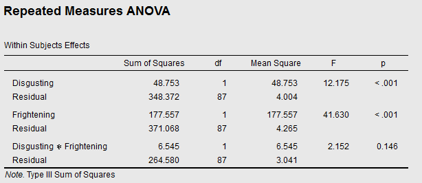
So there's a main effect of Disgusting (p < .001), indicating that people dislike disgusting bugs more than non-disgusting ones. And a main effect of Frightening (p < .001), indicating that people dislike frightening bugs more than non-frightening ones. There is no reliable Disgusting × Frightening interaction (p = 0.146), indicating that the two effects seem to be more or less additive.

If you've worked with Repeated Measures before, you probably know how to read a table like this.

Interpreting a Bayesian Repeated Measures with two factors

Now let's take a look at the Bayesian Repeated Measures for the same data:

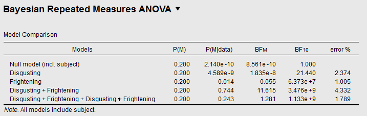
This table gives us 5 models. The first model is the null model, which embodies the null hypothesis (H0) that how much people dislike bugs doesn't depend on anything. The second model is one alternative hypothesis (HA), which embodies the hypothesis that how much people dislike bugs depends on how disgusting they are (but on nothing else). The BF10 column indicates how likely the data is under HA, compared to H0. In this case, the data is 21.44 times more likely under HA than under H0, corresponding to strong evidence for HA in favor of H0. In other words, there is strong evidence for an effect of Disgusting.

So far so good.

Things get tricky when you want to evaluate the evidence for the Disgusting × Frightening interaction: Does how much people dislike bugs depend on the interaction between how disgusting and how frightening they are? For example, perhaps people dislike all bugs more or less equally, except when they are both disgusting and frightening—maybe those bugs are disliked even more. That would be one possible interaction (you can think of others).

If you look at the last row, corresponding to the model with the interaction, you see a BF10 of about a billion. This means—this is worth repeating—that the data is a billion times more likely under this HA compared to H0.

Does this mean that there is strong evidence for the interaction? No! The reason that this model does so well is because of the two main effects, and not because of the interaction.

In order to evaluate the evidence for the interaction on its own, you need to compare the BF10 of the model with the interaction against the BF10 of the model with only the two main effects (i.e. everything except the interaction). If you do this, you see that the evidence for the interaction is 1.133 × 10^9 / 3.476 × 10^9 = 0.326. That is, there is substantial evidence against the interaction, as you would expect given the results from the traditional Repeated Measures.

Note that instead of dividing the values under BF10, you can also divide the values under P(M|data), which indicate the 'posterior' probability of the models after the data was collected. When comparing only two models, both approaches come down to the same thing (0.243 / 0.744 = 0.327). But when you compare more models, you need the P(M|data) column.

Interpreting a Bayesian Repeated Measures with many factors

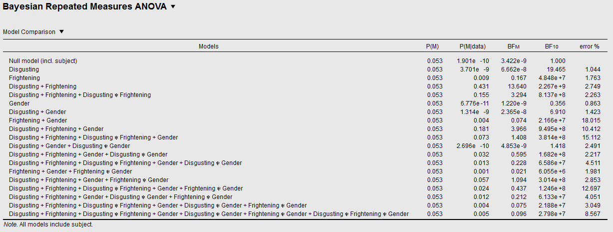
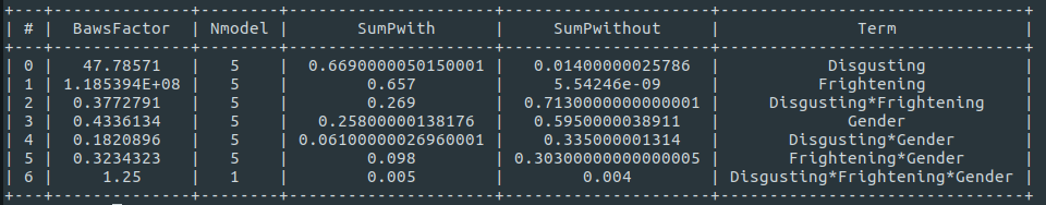
The nasty thing about model comparisons is that the number of models explodes when you add factors. To illustrate, let's see what happens when you add Gender as a (between-subject) factor. The model table for this three-factorial design looks like this:

Now say that you again want to quantify the evidence for the Disgusting × Frightening interaction. How can you do this? Which models should you compare?

Reasonable people may suggest different approaches. But here is one approach that I've labeled the Baws Factor, and that gives seemingly sensible results. The logic is as follows.

1. Determine your effect of interest. Here, this is Disgusting × Frightening.
2. Find all models that contain the effect of interest, but no interactions with the effect of interest. Let's call these the with models. Here, this means all models with the Disgusting × Frightening two-way interaction but without the Disgusting × Frightening × Gender three-way interaction.
3. From all the with models, strip the term of interest. Let's call the resulting models the without models. For example, the with model Disgusting + Frightening + Disgusting × Frightening is reduced to the without model Disgusting + Frightening.
4. The Baws factor is then the sum of P(M|data) of all with models, divided by the sum of P(M|data) of all without models.

Below, you can see all the models that are compared. The with models are indicated with a +. The without models are indicated with a -.

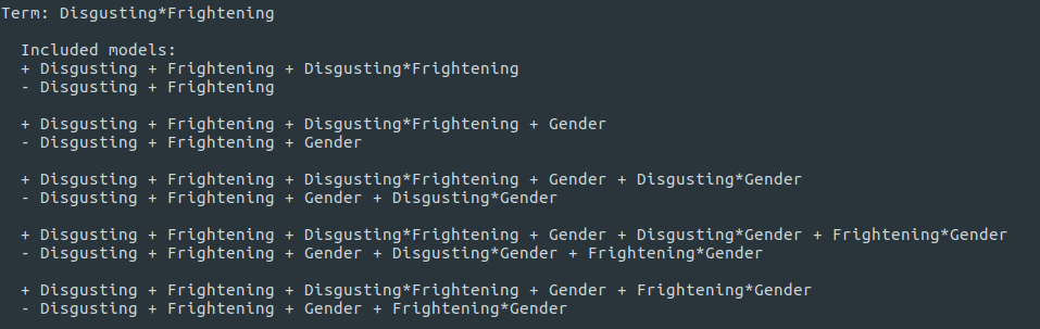
If you do the maths, the resulting Baws Factor for Disgusting × Frightening is 0.377. This is re-assuringly close to the result that we got for this interaction in the two-way Repeated Measures.

Unfortunately, JASP (0.8.1.1) does not yet allow you to automatically do these kinds of multiple-model comparisons. But this may come in the future releases, either in the form of the Baws Factor described here, or some variation of the same general idea.

What does the inclusion Bayes Factor mean?

If you know JASP, you may wonder how the Inclusion Bayes Factor, which you get if you tick the Effects box under Output, differs from the Baws Factor described above. Isn't the Inclusion Bayes Factor supposed to extract evidence for specific effects as well?

Let's take a look what the Inclusion Bayes Factors give us here:

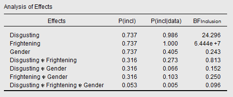
The Inclusion Bayes Factor for the Disgusting × Frightening interaction is 0.813. In other words, virtually no evidence for or against. Why is this different from our Baws Factor of 0.377? Which is correct?

Well, they are both correct, but reflect different things. The Inclusion Bayes Factor reflects, if my understanding is correct, the evidence for all models with a particular effect, compared to all models without that particular effect. But because all models that contain an interaction also contain the main effects of the interacting terms, the Inclusion Bayes Factor for an interaction also reflects the evidence for the main effects of the interacting terms.

You probably didn't get the preceding sentence. So let's rephrase: The Inclusion Bayes Factor for Disgusting × Frightening not only reflects the evidence for this interaction, but also for the main terms Disgusting and Frightening.

Personally, I find the Inclusion Bayes Factor hard to interpret, and I can't think of many situations in which it would be useful. But you may feel differently. The important thing is: Know which models you're comparing!